7 Inferential Statistics

In this chapter, we’ll explore the basics of inferential statistics, focusing on hypothesis testing and correlation analysis. We will walk through how to perform these tests in R, compare them to similar processes in SPSS, and understand how to interpret the results.

7.1 Hypothesis Testing

Hypothesis testing is a fundamental aspect of inferential statistics, allowing you to draw conclusions about populations based on sample data. In R, common hypothesis tests like t-tests, chi-square tests, and ANOVA are straightforward to perform. Let’s look at each in detail.

7.1.1 T-tests

A t-test is used to determine if there is a significant difference between the means of two groups. This test is equivalent to the COMPARE MEANS function in SPSS.

7.1.1.1 One-sample t-test

A one-sample t-test compares the mean of a single group against a known value (e.g., a population mean).

For example, let us look at the number of days each officer in the Serious Crime Unit has taken absence this year and compare it to the average number of days across all officers last year. We want to know if the mean differs from last year.

# Example: One-sample t-test
# Testing if the mean of a sample is significantly different from 50

data_officerabsencedays <- c(48, 50, 52, 51, 49, 47, 53, 50, 52, 48)

t.test(data_officerabsencedays, mu = 50)

## 
##  One Sample t-test
## 
## data:  data_officerabsencedays
## t = 0, df = 9, p-value = 1
## alternative hypothesis: true mean is not equal to 50
## 95 percent confidence interval:
##  48.56929 51.43071
## sample estimates:
## mean of x 
##        50

7.1.1.2 Independent two-sample t-test

An independent t-test compares the means of two independent groups.

For example, let us review the Stop and Search data for Merton and Kingston across a 6 month period. We want to know if the average number of stop and searches differs between the two boroughs.

# Example: Independent two-sample t-test
# Comparing scores of two independent groups

data_stopsearch_merton <- c(53, 55, 68, 65, 72, 63)
data_Stopsearch_kingston <- c(59, 69, 65, 70, 75, 67)

t.test(data_stopsearch_merton, data_Stopsearch_kingston)

## 
##  Welch Two Sample t-test
## 
## data:  data_stopsearch_merton and data_Stopsearch_kingston
## t = -1.2967, df = 9.1156, p-value = 0.2266
## alternative hypothesis: true difference in means is not equal to 0
## 95 percent confidence interval:
##  -13.249305   3.582638
## sample estimates:
## mean of x mean of y 
##  62.66667  67.50000

7.1.1.3 Paired t-test

A paired t-test compares means from the same group at different times (e.g., before and after a treatment).

# Example: Paired t-test
# Comparing pre- and post-treatment scores for the same group
pre_treatment <- c(100, 102, 104, 106, 108)
post_treatment <- c(110, 111, 115, 117, 120)
t.test(pre_treatment, post_treatment, paired = TRUE)

## 
##  Paired t-test
## 
## data:  pre_treatment and post_treatment
## t = -20.788, df = 4, p-value = 3.164e-05
## alternative hypothesis: true mean difference is not equal to 0
## 95 percent confidence interval:
##  -12.015715  -9.184285
## sample estimates:
## mean difference 
##           -10.6

7.1.1.4 Interpreting T-Test Results

T-Value: Indicates the size of the difference relative to the variation in your sample data.
P-Value: Tells you whether the observed difference is statistically significant. A p-value less than 0.05 typically indicates statistical significance.
Confidence Interval: Provides a range within which the true population parameter is likely to fall.

In SPSS, p-values and confidence intervals are found in the output tables after running the analysis. In R, they appear in the results from the t.test() function.

Exercise!

The Metropolitan Police Service have implemented a new strategy to target Violence Against Women and Girls in 5 wards. The number of incidents in March across these 5 wards was 100, 102, 104, 106, and 108. After the implementation of the new strategy the number of incidents in April across these 5 wards was 110, 111, 115, 117, 120 respectively. Has the new strategy had an impact on the number of incidents?

7.1.2 Chi-square Tests

Chi-square tests assess the relationship between categorical variables. In SPSS, this corresponds to the CROSSTABS function with the “Chi-square” option.

7.1.2.1 Chi-Square Test of Independence

The Chi-Square Test of Independence tests if two categorical variables are independent. For example, you might want to determine if there is an association between the type of crime and the borough where the crime occurred.

# Example: Chi-square test
# Testing the association between two categorical variables

# Example data: Crime frequencies in different boroughs
crime_data <- matrix(c(
  100, 50, 30,   # Borough 1: Crime Type A, B, C
  80, 40, 20,    # Borough 2: Crime Type A, B, C
  70, 30, 25     # Borough 3: Crime Type A, B, C
), nrow = 3, byrow = TRUE)

# Add row and column names
rownames(crime_data) <- c("Borough 1", "Borough 2", "Borough 3")
colnames(crime_data) <- c("Crime Type A", "Crime Type B", "Crime Type C")

# Perform the Chi-Square Test of Independence
chisq_test_independence <- chisq.test(crime_data)

# Print the results
print(chisq_test_independence)

## 
##  Pearson's Chi-squared test
## 
## data:  crime_data
## X-squared = 1.9076, df = 4, p-value = 0.7527

7.1.2.2 Chi-Square Goodness-of-Fit Test:

The Chi-Square Goodness-of-Fit Test tests if a single categorical variable follows a specific distribution. For example, suppose you have observed the frequency of crimes across different types, and you want to test if these frequencies are uniformly distributed.

# Example: Chi-square test
# Testing the distribution of a categorical variable

# Example data: Observed frequencies of crime types
observed_frequencies <- c(100, 150, 80, 70)  # Frequencies of Crime Type A, B, C, D

# Expected frequencies under the null hypothesis (uniform distribution)
expected_frequencies <- rep(sum(observed_frequencies) / length(observed_frequencies), length(observed_frequencies))

# Perform the Chi-Square Goodness-of-Fit Test
chisq_test_goodness_of_fit <- chisq.test(observed_frequencies, p = rep(1/length(observed_frequencies), length(observed_frequencies)))

# Print the results
print(chisq_test_goodness_of_fit)

## 
##  Chi-squared test for given probabilities
## 
## data:  observed_frequencies
## X-squared = 38, df = 3, p-value = 2.826e-08

7.1.2.3 Interpreting Chi-Square Test Results

Chi-Square Statistic: Measures the deviation of observed frequencies from expected frequencies.
P-Value: Indicates whether the association or distribution is statistically significant. A p-value less than 0.05 suggests a significant result.
Degrees of Freedom (df): The number of independent values in the test, affecting the chi-square distribution.

In SPSS, p-values and confidence intervals are found in the output tables after running the analysis. In R, they appear in the results from the chisq.test() function.

Exercise!

You want to identify if the number of Stop and Search performed in the month of September across 6 Boroughs where the Stop and Search occurred is Uniformly distributed. Use the following data to identify if the Number of Stop and Search performed is uniform across the 6 Boroughs.

Richmond: 36 // Kingston: 25 // Merton: 28 // Sutton: 34 // Croydon: 42 // Wandsworth: 32

7.1.3 ANOVA (Analysis of Variance)

ANOVA tests are used to compare the means of three or more groups. This is analogous to the ONE-WAY ANOVA function in SPSS.

For example, let us review the number of crimes reported in three geographic areas over a four week period. We will perform a one-way ANOVA to determine if there are significant differences in the average number of crimes reported across these districts.

# Example: One-way ANOVA
# Comparing scores across three different groups

ward1 <- c(150, 155, 160, 158) #Ward 1
ward2 <- c(163, 165, 172, 174) #Ward 2
ward3 <- c(178, 172, 183, 153) #Ward 3

data <- data.frame(
  score = c(ward1, ward2, ward3),
  group = factor(rep(1:3, each = 4))
)
anova_result <- aov(score ~ group, data = data)
summary(anova_result)

##             Df Sum Sq Mean Sq F value Pr(>F)  
## group        2  559.5  279.75   3.822 0.0629 .
## Residuals    9  658.7   73.19                 
## ---
## Signif. codes:  0 '***' 0.001 '**' 0.01 '*' 0.05 '.' 0.1 ' ' 1

7.1.3.1 Interpreting ANOVA Results

F-Value: Indicates the ratio of variance between the groups to the variance within the groups. A higher F-value suggests a greater likelihood that the group means are different.
P-Value: Indicates whether the group means are significantly different. A p-value less than 0.05 usually suggests that there is a significant difference among group means.

In SPSS, p-values and confidence intervals are found in the output tables after running the analysis. In R, they appear in the results from the summary() function for ANOVA.

7.1.3.2 Post-Hoc ANOVA Analysis (if significant)

If the ANOVA test is significant, you may want to perform a post-hoc test to identify which specific groups differ from each other. A common post-hoc test is Tukey’s Honest Significant Difference (HSD) test.

# Perform Tukey's HSD test for post-hoc analysis
tukey_result <- TukeyHSD(anova_result)

# Print the results of Tukey's HSD test
print(tukey_result)

##   Tukey multiple comparisons of means
##     95% family-wise confidence level
## 
## Fit: aov(formula = score ~ group, data = data)
## 
## $group
##      diff        lwr      upr     p adj
## 2-1 12.75  -4.140416 29.64042 0.1431152
## 3-1 15.75  -1.140416 32.64042 0.0670591
## 3-2  3.00 -13.890416 19.89042 0.8750277

Interpreting Tukey’s HSD Results

Pairwise Comparisons: Tukey’s HSD provides pairwise comparisons between all groups. Significant differences are indicated where the confidence intervals for the difference between group means do not contain zero.
Adjusted p-Values: The test adjusts for multiple comparisons to control the family-wise error rate.

Exercise!

Local residents in 3 boroughs were asked to rate their confidence in the Metropolitan Police Service rating their scores from 0 to 10. The average score across a 3 month period is as follows.

Kingston : 7.0, 7.5, 8.2
Richmond : 8.3, 6.4, 7.9
Sutton : 6.4, 4.5, 5.8

Does the mean confidence level across the 3 month preiod differ between the three boroughs?

7.2 Correlation Analysis

Correlation analysis measures the strength and direction of the relationship between two variables. The most common methods are Pearson and Spearman correlations, which are available in both SPSS and R.

7.2.1 Pearson Correlation

The Pearson correlation measures the linear relationship between two continuous variables. It’s equivalent to BIVARIATE CORRELATIONS in SPSS.

For example, suppose you have data on the number of crimes reported and the number of police patrol hours in different beats and you want to see if there’s a linear relationship between these two variables.

# Example: Pearson correlation
# Measuring the correlation between two continuous variables

# Create example data: Crime rate and police patrol hours
data_beat <- data.frame(
  patrol_hours = c(20, 30, 25, 40, 35, 45, 50, 60, 55, 65),  # Hours of patrol
  crime_rate = c(15, 22, 18, 25, 20, 30, 28, 35, 32, 40)     # Number of crimes
)

# View the dataset
print(data_beat)

##    patrol_hours crime_rate
## 1            20         15
## 2            30         22
## 3            25         18
## 4            40         25
## 5            35         20
## 6            45         30
## 7            50         28
## 8            60         35
## 9            55         32
## 10           65         40

cor(data_beat$patrol_hours, data_beat$crime_rate, method = "pearson")

## [1] 0.9766032

Interpreting Pearson Correlation

Correlation Coefficient (r): Ranges from -1 to 1. A value close to 1 indicates a strong positive correlation, while a value close to -1 indicates a strong negative correlation. A value around 0 suggests no linear correlation.
P-Value: Tests if the observed correlation is significantly different from zero.

In SPSS, the correlation coefficient and p-value are reported together in a table. In R, these can be accessed using the cor.test() function if you need detailed statistical outputs.

7.2.2 Spearman Correlation

Spearman correlation is a non-parametric measure of rank correlation, useful when the data is not normally distributed or the relationship is not linear.

We will use the same dataset to see if there is a monotonic relationship between crime rates and patrol hours.

# Example: Spearman correlation
# Measuring the correlation between two variables using ranks
cor(data_beat$patrol_hours, data_beat$crime_rate, method = "spearman")

## [1] 0.9757576

Interpreting Spearman Correlation

Spearman’s Rank Correlation Coefficient (ρ): Ranges from -1 to 1, similar to Pearson. It measures how well the relationship between two variables can be described by a monotonic function.

In SPSS, the correlation coefficient and p-value are reported together in a table. In R, these can be accessed using the cor.test() function if you need detailed statistical outputs.

7.2.3 Pearson vs Spearman?

Pearson’s correlation coefficient is used when you want to measure the strength and direction of a linear relationship between two continuous variables that are normally distributed. It assesses how well the relationship between the variables can be described by a straight line. Use Pearson’s correlation when the data is interval or ratio and there is a linear relationship.

Spearman’s rank correlation coefficient is suitable when the relationship between the variables is monotonic but not necessarily linear, or when the data does not meet the assumptions required for Pearson’s correlation, such as normality or interval scale. Spearman’s correlation assesses how well the relationship between the variables can be described by a monotonic function, which means it evaluates whether higher ranks in one variable correspond to higher ranks in another, regardless of the exact form of the relationship.

In summary, use Pearson’s correlation for linear relationships with continuous data and Spearman’s correlation for monotonic relationships or when data is ordinal or not normally distributed.

7.2.4 Visualising Correlations

Visualising correlations can help in understanding the relationship between multiple variables. The corrplot package in R provides a convenient way to create correlation matrices.

Using the same beat dataset used above.

# Example: Correlation matrix visualization
# Creating and visualizing a correlation matrix
library(corrplot)

## corrplot 0.94 loaded

# Compute the correlation matrix
cor_matrix <- cor(data_beat)

# Visualize the correlation matrix
corrplot(cor_matrix, method = "circle")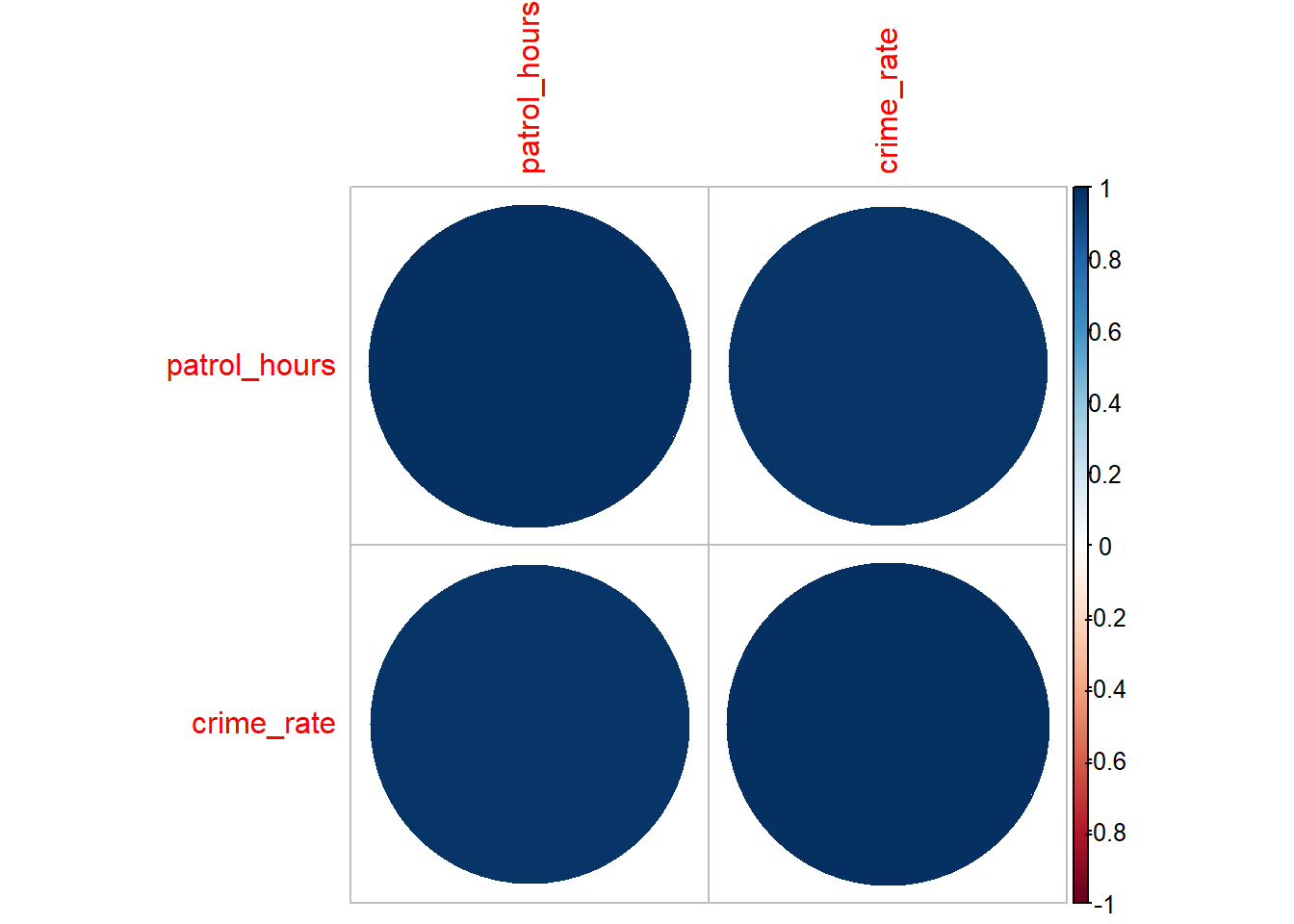

Interpreting the Correlation Matrix Plot

Colours and Sizes: Represent the strength and direction of the correlation. Positive correlations are typically shown in one colour and negative correlations in another.
Magnitude of Correlation: Larger circles or stronger colours indicate stronger correlations.

Exercise!

You have data on the number of community outreach programs conducted in 6 boroughs as well as the associated crime rates. You want to determine if there’s a linear relationship between these two variables. Use the data below to perform a correlation analysis.

Borough	Community Programs	Number of Crimes
Kingston	4	145
Merton	5	154
Sutton	8	218
Croydon	19	255
Lambeth	17	234
Wandsworth	15	189

7.3 Conclusion

In this chapter, you’ve learned how to perform common inferential statistical tests in R, including t-tests, chi-square tests, and ANOVA, as well as how to conduct and visualise correlation analyses. Each test has an equivalent function in SPSS, but R provides more flexibility and control over the analysis process. This chapter has laid the groundwork for applying these techniques to your own data analyses, building on your existing knowledge from SPSS.