2 Getting Started with R
2.1 The R Environment
2.1.1 Overview of the RStudio Interface
RStudio is a powerful integrated development environment (IDE) that provides a user-friendly interface for working with R. Understanding its layout will help you navigate and utilise its features effectively.
Script Editor: This is where you write and save your R scripts. You can execute lines of code or entire scripts from here.
Console: The Console displays the output of your commands and allows you to run R code directly. It’s useful for quick calculations and immediate feedback.
Environment/History Pane: The Environment pane shows the objects (e.g., data frames, variables) in your current R session. The History tab logs commands you’ve executed.
Files/Plots/Packages/Help Pane: This multi-functional pane lets you manage files, view plots, install/load packages, and access R’s help system.
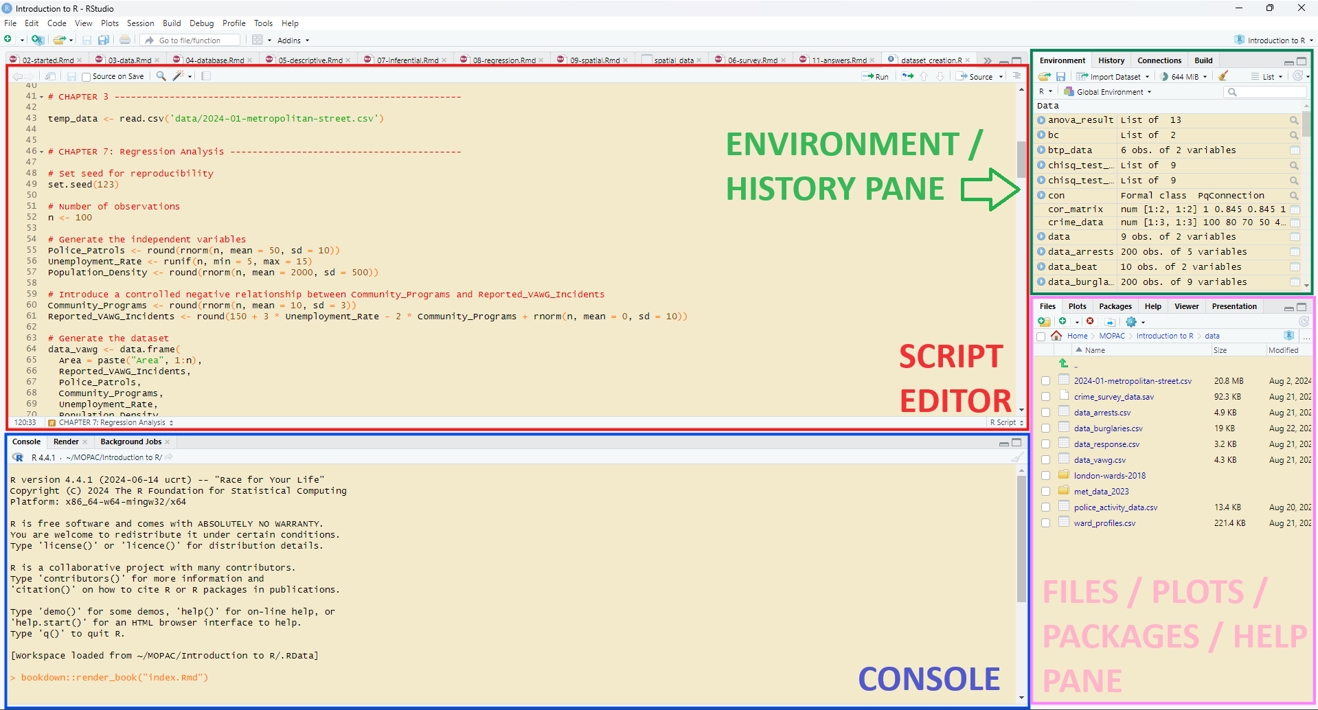
Figure 2.1: RStudio IDE Layout
2.1.2 Console vs. Scripts vs. Notebooks
- Console: Ideal for quick calculations and testing small pieces of code. Commands typed here are executed immediately.
- Scripts: These are text files with R code that you can save and run as needed. Scripts are useful for documenting your workflow and making analyses reproducible.
- Notebooks: R Notebooks combine code, output, and markdown text in one document. They are great for creating interactive reports and combining narrative with code.
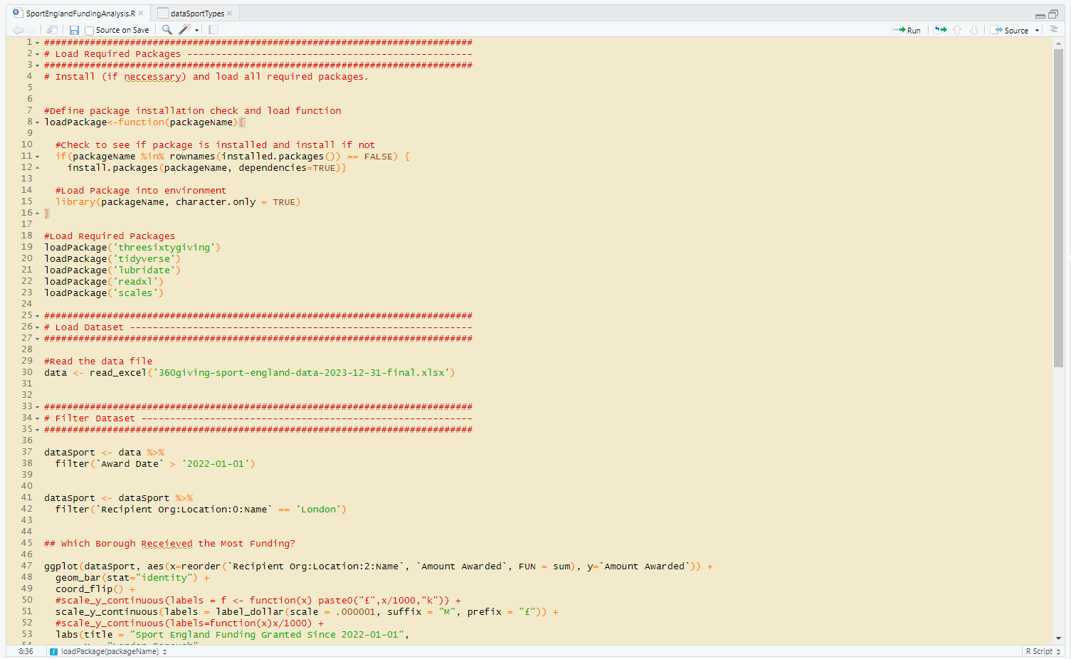
Figure 2.2: Example R Script
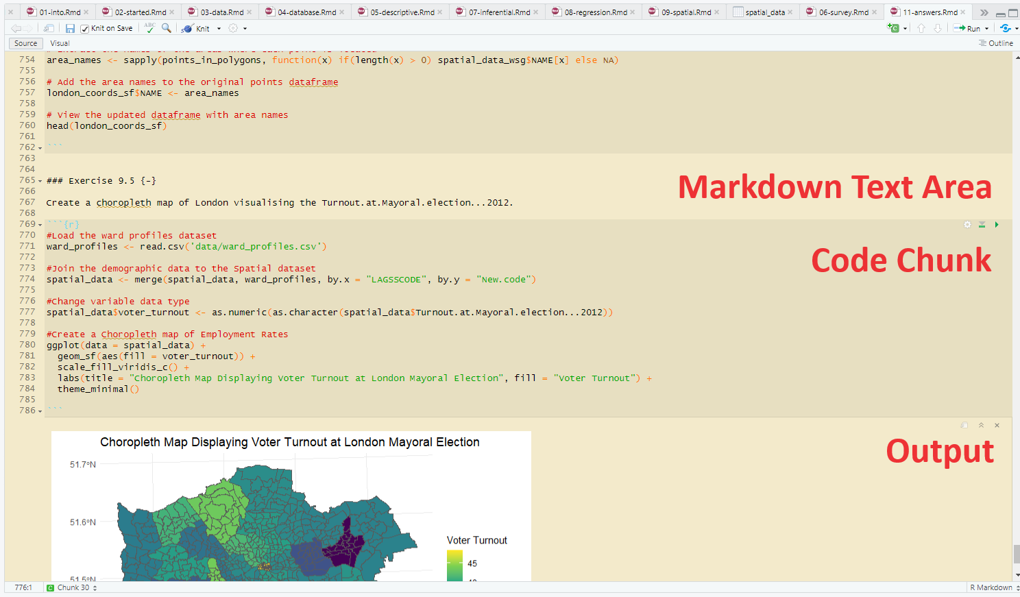
Figure 2.3: Example R Notebook with Text, Code, and Output Areas Labelled
2.2 Introduction to R Packages and Installing Key Packages
R comes with a robust set of core functions that allow you to perform a wide range of statistical analyses and data manipulations. However, the true power of R lies in its extensive ecosystem of packages, which extend its functionality far beyond the basics. These packages, developed by the global R community, enable users to perform specialised tasks, from advanced statistical modelling and machine learning to data visualisation and spatial analysis. Understanding how to install and use these packages is key to unlocking the full potential of R.
2.2.1 Introduction to R Packages
A package in R is a collection of functions, data, and documentation that extends the base functionality of R. There are thousands of packages available, each designed to solve specific problems or add capabilities to your R environment.
Using packages allows you to leverage the work of other developers and statisticians, saving you time and effort.
2.2.2 Installing and Loading Packages
To use a package in R, you first need to install it, and then load it into your current R session. Packages are typically installed from the Comprehensive R Archive Network (CRAN), which is the primary repository for R packages.
Installing a Package
To install a package, use the install.packages() function. For example, to install the ggplot2 package, which is used for creating visualisations, you would run:
This command downloads the package from CRAN and installs it on your system. You only need to install a package once on your machine.
Loading a Package
Once a package is installed, you need to load it into your current R session using the library() function. For example:
After loading the package, you can use its functions in your R code.
Installing Multiple Packages at Once
You can install multiple packages at once by passing a vector (we will come onto these later!)
of package names to install.packages():
This is useful when you’re setting up a new R environment or working on a project that requires several packages.
2.2.3 Key Packages for Data Analysis
For those transitioning from SPSS to R, here are some key packages you’ll frequently use:
tidyverse: A collection of packages for data manipulation, exploration, and visualisation. It includes packages like dplyr, ggplot2, tidyr, and readr.haven: Used to import and export SPSS, Stata, and SAS files. This package is essential for working with data originally created in SPSS.dplyr: A package for data manipulation. It provides functions for filtering, selecting, and transforming data, making it easier to manage datasets.ggplot2: A powerful package for creating complex visualisations. It is part of the tidyverse and is widely used for creating a variety of plots.readr: For importing and exporting CSV and other flat files. It provides functions that are faster and more flexible than base R’s equivalent functions.sf: If you are working with spatial data,sfis essential. It provides a simple feature (sf) framework for handling and analysing spatial data.survey: For survey data analysis. This package provides tools for analysing complex survey samples, including handling survey weights.psych: Useful for psychological research and other fields involving human behaviour. It provides tools for descriptive statistics, factor analysis, and more.
2.2.4 Managing Package Dependencies
When working with projects, it’s important to manage package dependencies to ensure that your code runs smoothly on different systems. Consider using the renv package to manage project-specific dependencies. This package allows you to create isolated environments for your R projects, ensuring that the correct versions of packages are used.
2.2.5 Summary
R packages are a cornerstone of efficient and effective data analysis in R. Understanding how to install and load packages, as well as identifying key packages for your analysis, will significantly enhance your ability to work with data in R. By mastering packages, you unlock the full potential of R and make your workflow more powerful and streamlined. Throughout this book we will utilise a number of packages so make sure you are familiar with installing and loading different packages.
2.3 Coding Conventions and Best Practices
In this section we briefly touch on coding conventions and best practices. However, we recommend you check out our other book on the Best Coding Practices in R.
2.3.1 Writing Clean and Readable Code
Good coding practices enhance readability and maintainability. Here are some guidelines:
Use Descriptive Names: Choose meaningful variable and function names that describe their purpose.
Consistent Indentation: Indent your code consistently to improve readability.
2.4 Data Types and Structures
2.4.1 Introduction to Vectors, Data Frames, Lists, and Factors
Vectors: A sequence of elements of the same type. Examples include numeric, character, and logical vectors.
# Numeric vector
numbers <- c(1, 2, 3, 4, 5)

# Character vector
names <- c("Alice", "Bob", "Charlie")
Data Frames: Two-dimensional tables where each column can be of a different type. Data frames are similar to SPSS datasets.
# Creating a data frame
df_offenders <- data.frame(OffenderName = c("Alice", "Bob"), OffenderAge = c(25, 30))
Lists: Collections of objects that can be of different types, including other lists.
Factors: Used for categorical data. They store both the values and the corresponding levels.
2.4.2 Comparing R Data Types to SPSS Data Types
In SPSS:
- Variables can be numeric, string, or categorical.
- Data Structures include datasets, which are similar to R data frames.
In R:
- Vectors are like SPSS variables.
- Data Frames are akin to SPSS datasets, with columns of different types.
- Lists provide more flexibility compared to SPSS’s data structures.
- Factors are used for categorical data, similar to SPSS’s categorical variables.
2.5 Basic Operations and Functions in R
2.5.1 Arithmetic Operations
R performs basic arithmetic operations similarly to SPSS. Examples include addition, subtraction, multiplication, and division.
# Arithmetic operations
addition <- 5 + 3
subtraction <- 10 - 4
multiplication <- 7 * 2
division <- 8 / 2
exponentiation <- 2^3
Exercise!
Execute these operations in R and compare with results from SPSS’s Compute function. Can you do this in both the console and the script editor?
2.5.2 Logical Operations
Logical operations include comparisons like equality and inequality, as well as logical operators such as AND and OR.
# Logical operations
equal <- (5 == 5)  # TRUE
not_equal <- (5 != 3)  # TRUE
greater_than <- (5 > 3)  # TRUE
and_operation <- (5 > 3 & 4 < 6)  # TRUE
or_operation <- (5 > 6 | 4 < 6)  # TRUE
Exercise!
Test these logical operations in R and compare them to SPSS’s logical operators.
2.5.3 Basic Functions
R includes many built-in functions for statistical calculations, data manipulation, and more. Common functions include mean(), sd(), sum(), and length().
# Basic functions
data <- c(1, 2, 3, 4, 5)
mean_value <- mean(data)
sd_value <- sd(data)
total_sum <- sum(data)
data_length <- length(data)
Exercise!
Between January 2023 and December 2023 the number of Violent and Sexual Offences in Wandsworth were as follows: 568, 568, 603, 604, 685, 871, 697, 608, 657, 681, 630, and 720. (1) Create a vector representing the number of Violent and Sexual Offences in Wandsworth. (2) What was the mean number of crimes each month? (3) What was the total number of crimes across the year? (4) What is the length of the vector?
2.6 Conclusion
In this chapter, you’ve learned about the RStudio interface, how to import data from SPSS, coding conventions, and the basics of R data types, structures, and operations. With this foundation, you’re prepared to start working with data in R and leveraging its powerful capabilities for analysis. In the next chapter, we’ll delve into more advanced data manipulation techniques to further enhance your skills.